Non-equilibrium thermodynamics and the folding of biomolecules
The Jarzynski Equality and Crooks Fluctuation theorem and their experimental verification
This is the paper I wrote as part of the requirements for my Comps II exam (aka Master’s exam) in the Physics Department at CU Boulder. The talk slides can be found here.
In the second half of the 19th century, thermodynamics was formalized with a statistical mechanics foundation by Boltzmann, Maxwell, Gibbs, and others. However, the only known relations for non-equilibrium systems were given by inequalities until the 1990s, when several remarkable exact results were found which hold for systems arbitrarily far from equilibrium such as the Jarzynski equality and Crooks fluctuation theorem. Around the same time, the ability to manipulate complex molecular systems using optical tweezers was rapidly advancing. Using colloidal particles and strands of RNA manipulated via optical tweezers, both Jarzynski’s and Crooks’ results were soon experimentally verified. We review the Jarzynski equality and Crooks fluctuation theorem and their experimental verification. This review will include derivations with the goal of clearly demonstrating how each result is applied to the experimental setting of pulling on molecules trapped in optical tweezers. To aid in this goal, we introduce a simple toy Monte Carlo model, inspired by the one used in Crooks’ original paper, implemented in simple, self-contained Julia code provided in the appendices. Crucially, this toy model concretely illustrates how free energy landscapes can be extracted from data taken in non-equilibrium experiments and the differences in experimental settings and accuracy between the Jarzynski equality and Crooks fluctuation theorem.
Introduction
In Erwin Schrödinger’s 1944 book titled What Is Life? he ponders the apparent paradoxes of life if one naively applies the laws of thermodynamics to biological systems (Schrödinger 1992; Phillips 2021). One of these apparent paradoxes is that of “order from disorder”: how can biological systems maintain their ordered, low entropic state in spite of the second law of thermodynamics? Obviously, this is the result of such systems not being isolated and having a continuous supply of free energy with which to do their work; thus life cannot be described by quasi-static equilibrium thermodynamic processes.
We also have the question of the scale at which biological systems are able to maintain order. Naively, one might expect “small” systems to be incapable of maintaining order over long time scales as the \(1/\sqrt{N}\) thermodynamic fluctuations for only a few hundred atoms would be significant. Understanding the rates at which processes happen on biomolecular scales requires understanding the free energy landscape of complex biomolecules. Yet, without the law of large numbers which thermodynamics relies on for its exacting precision at macroscopic scales, can we hope to establish exact relations for such apparently stochastic dynamics?
Resolving such apparent paradoxes requires relaxing the equilibrium assumption and deriving non-equilibrium thermodynamic relations which take into account the stochastic nature of fast-driven dynamics. Two such important relations are the closely related Jarzynski equality (JE) and Crooks fluctuation theorem (CFT), which relate the work for a process to the free energy difference between the initial and final states where the system need not be in thermodynamic equilibrium during the process (Jarzynski 1997; Crooks 1999).
By measuring the work exerted to unfold and refold a biomolecule, the JE and CFT can be used to find the free energy landscape of the molecule. This energy landscape helps us to understand the thermodynamic stability of these biological molecules and how transformations between their various configurations are driven by the non-equilibrium processes that sustain life. This ultimately helps further our understanding of the mechanisms behind the “order from disorder” paradoxes that Schrödinger pondered.
This paper will begin by briefly discussing the motivating case of unfolding an RNA hairpin while quickly introducing the requisite definitions of quantities from thermodynamics and statistical mechanics in Motivation and a brief review of equilibrium thermodynamics. Then The toy model will introduce a toy Monte Carlo simulation designed to capture relevant features of the RNA hairpin unfolding experiment and the difference between the equilibrium and non-equilibrium regimes. The Jarzynski equality will then apply the JE to this toy model. Next, The Crooks fluctuation theorem will demonstrate how the JE follows from the CFT and will also apply the CFT to the toy model. Having used the toy model to illustrate how the JE and CFT can be applied in practice to both computational and experimental data, Optical tweezer experiments will then present data from two foundational experiments which pull on RNA hairpins with optical tweezers in order to experimentally verify the JE and CFT.
A proof of the CFT is presented in Appendix: Proof of the Crooks fluctuation theorem while Appendix: Julia code reproducing Crooks’ original NESS toy model contains code written in Julia which implements the toy model in Crooks’ original paper and reproduces several of the plots in that paper. Appendix: Julia code implementing the RNA folding inspired toy model then contains the Julia code that implements toy model presented in The toy model which was inspired by Crooks’ original toy model. These toy models are pedagogically valuable as their implementations take less than 100 lines of code and do not rely on any external packages.
Motivation and a brief review of equilibrium thermodynamics

Consider an RNA hairpin, illustrated in Fig. 1, to which enough force is applied to the ends such that the hairpin structure is pulled apart leaving just a straight, single strand of RNA. Both the folded and unfolded configurations are stable, however it takes some amount of work to go from one to the other. Based on intuition about the electrostatic forces involved in hydrogen bonding, we might correctly guess that the folded configuration is at a lower potential energy than the unfolded. Thus we can sketch what the energy landscape of this RNA hairpin may look like to first approximation.

Fig. 2 shows what we might expect, where the coordinate along which the potential energy changes is the extension or distance between the ends of the RNA strand. The actual configuration space of the biomolecule is incredibly complex and high-dimensional, but by picking out extension as a single reaction coordinate along which energy landscape is averaged, we greatly simplify the problem. However, due to all the complex atomic interactions that give rise to this complex and high-dimensional energy landscape, it is impossible to analytically compute exactly what this energy landscape looks like and thus we cannot a priori determine the energy difference \(\Delta E\) between the folded and unfolded configurations. Yet knowing the value of \(\Delta E\) is incredibly useful for understanding what biological process can and cannot occur and how fast they may occur. So we are left with attempting to determine \(\Delta E\) either experimentally or computationally.
At this point it worth explicitly mentioning that when properties of these biomolecular structures are discussed, such as \(\Delta E\), it is almost always implicitly assumed that they are contained within some aqueous solution. This assumption carries along with it the notion that these molecules are always coupled to some large heat bath and thus should be considered as thermodynamic systems whose equilibrium behavior is described by the canonical partition function
\begin{align} Z=\sum_x e^{-\beta E(x)} \end{align}where \(\beta = 1/k_B T\) with \(k_B\) being the Boltzmann constant and \(T\) the temperature. Thus, an experiment which quasi-statically (in this case isothermally) moves between the two configurations, \(A\) and \(B\), will actually be measuring the free energy difference \(\Delta F\) between them, not the potential energy difference \(\Delta E\), due to the presence of the heat bath. The statistical mechanics definition of the (Helmholtz) free energy of a given configuration is
\begin{align} \label{eq:free-energy-sm} F_A = -k_B T\ln Z_A\; . \end{align}Using the first law of thermodynamics, \(\dd{E} = \delta W + \delta Q\), where the work \(W\) and heat \(Q\) follow the sign convention that positive means energy flow into the system, along with the second law defining entropy as \(\dd{S} = \frac{1}{T}\delta Q\), we have that
\begin{align} \delta W = \dd{(E - TS)} + S\dd{T} = \dd{(E[T])} + S\dd{T} \end{align}where \(E[T]\) denotes the Legendre transform of \(E\). This defines the free energy \(F\equiv E[T]\) in thermodynamics and can be shown to correspond to the statistical mechanics definition in Eq. \eqref{eq:free-energy-sm} (Swendsen 2019). Thus, for a quasi-static process from \(A\) to \(B\) where the system remains at constant temperature, the work is simply the free energy difference: \(W = F_B - F_A\).
However, if \(A\) and \(B\) are not connected via a quasi-static process, meaning that the system is not in equilibrium at every point between \(A\) and \(B\), then the second law states that \(\dd{S} > \frac{1}{T}\delta Q\) and the maximum work principle immediately follows
\begin{align} \label{eq:max-work} W > F_B - F_A\; . \end{align}The breakthrough of Jarzynski and Crooks was to strengthen this inequality to an equality which holds for arbitrary non-equilibrium paths from \(A\) to \(B\).
Before introducing these non-equilibrium results of Jarzynski and Crooks, it’s worth discussing what types of non-equilibrium systems we might be able to consider and how we can gain access to information about them as non-equilibrium dynamics can, in general, be arbitrarily complex. Given the inherently stochastic nature of thermodynamic systems, measuring properties of these systems accurately requires either performing many identical experiments and doing statistical analysis, or having the measurement instrument itself perform the averaging itself by interacting with the system for long enough times such that fluctuations become negligible. In a typical equilibrium thermodynamics experiment, these two ways of measuring the system are equivalent. Due to the equilibrium assumptions of ergodicity and Boltzmann distributed probabilities, the statistical average of many identical experiments is equivalent to a longer measurement which averages over the thermodynamic fluctuations However, when considering measuring properties of non-equilibrium systems, these two ways of measuring a system are no longer equivalent. There are two concrete experimental settings which illustrate this point and for which exact non-equilibrium relations are known. These relations allow non-equilibrium measurements to be related to quantities only defined at equilibrium, such as the free energy.
The first experimental setting applies to what are known as a non-equilibrium steady states (NESSs). In a NESS, a system is subject to a fast enough force that is periodic in time so that a NESS cannot every relax to an equilibrium state. However after sufficiently many periods of the force, the system will relax into a steady state distribution. Such systems are amenable to being measured in either of the ways described above, however the arithmetic mean of many measurements will not necessarily correspond to a longer measurement unless they each correspond to time intervals which are integer multiples of the period.
The second experimental setting consists of driving a system from equilibrium for some finite duration of time then stopping. In this experimental setting, its possible that each run is sufficiently stochastic and/or that the system takes an unknown amount of time to relax into equilibrium. In such settings there may be no way to relate an ensemble of measurements at short times to fewer measurements at some arbitrary, longer time after the drive is turned off. The motivating example of understanding the free energy difference between unfolded and folded configurations of an RNA hairpin fall into this second experimental setting. Both the JE and the CFT can be applied to this setting as we will illustrate with a toy model in the remaining sections. However, the its worth noting that the JE is not applicable to the setting of NESSs while the CFT is.
The toy model
In Crooks original paper, he introduces a simple, discrete model consisting of a linear potential on 32 states with periodic boundary conditions which is continuously driven in one direction. This model offers pedagogical value in illustrating the application of CFT to a simple, yet physically relevant system. In Appendix Appendix: Julia code reproducing Crooks’ original NESS toy model we implement Crooks original simple model and reproduce several of the plots in the paper (Crooks 1999). However, Crooks’ simple model only demonstrates the applicability of Crooks’ fluctuation theorem to a system in a NESS. While NESSs are very relevant to many experiments, such as dragging a colloidal particle through a solution (Wang et al. 2002), they are not directly relevant to the typical experimental setting of pulling on biomolecules.
Inspired by this model and its pedagogical value, we now introduce a similar toy model based on the schematic energy landscape shown in Fig. 2 that we expect for the process of RNA hairpin unfolding and refolding. This toy model will then help make the non-equilibrium results of Jarzynski and Crooks more concrete by illustrating how they are applied in experiments which pull on biomolecular structures.

Like in Crooks’ model, this toy model consists of a discrete state space of 32 positions which are meant to be analogous to the distance between the ends of the RNA strand. However, unlike Crooks’ model, we consider hard boundaries such the system can only move right from \(x=1\) and left from \(x=32\). To capture non-equilibrium behavior, we model a driving force which modifies the potential energy of each state in discrete steps from \(\lambda=1\) to \(\lambda=29\). Fig. 3 illustrates the energy landscape of this model at \(\lambda=1,15,29\). At \(\lambda=1\) there is a linear potential with a degenerate ground state with \(E(x=9) = E(x=10) = 0\). From \(\lambda=2\to 14\), the energy of this ground state increases while another local minima forms with \(E(x=23) = E(x=24) = 14\) until at \(\lambda=15\) the double wells have equal energy. From \(\lambda=16\to 29\), the right well is the ground state and finally by \(\lambda=29\) there is no left well. Since the shape of the potential at the start (\(\lambda=1\)) and the end (\(\lambda=29\)) are related by mirror reflection about \(x=16\) and a y-shift of \(14\), the free energy difference between the two configurations must be \(\Delta F = F_{\lambda=29} - F_{\lambda=1} = 14\beta\). Thus, we expect that a quasi-static process which goes from \(\lambda=1\) to \(\lambda=29\) while maintaining thermal equilibrium would take work \(W=14\beta\). Fig. 4. plots the free energy at several values of \(\lambda\). Note that all the plots presented in this paper are at temperature \(\beta=1/2\).

The equilibrium probability distribution at each \(\lambda\) is given by the Boltzmann factor normalized by the partition function or equivalently the difference between free energy and internal energy (Swendsen 2019)
\begin{align} \label{eq:pr-config} P(x|\lambda) &= \frac{1}{Z} e^{-\beta E_\lambda(x)} = e^{\beta F_\lambda - \beta E_\lambda(x)} \end{align}This can be analytically computed for this toy model and is also plotted in Fig. 3 for several values of \(\lambda\). However, in order to obtain non-equilibrium probability distributions we will need to turn to numerics such as Markov chain Monte Carlo (MCMC) methods. Perhaps the simplest MCMC method is the Metropolis algorithm (Metropolis et al. 1953) which is what Crooks originally used and we will also use here. Before turning to non-equilibrium simulations, its always good to check the code against known analytical expressions which Fig. 3 also demonstrates by plotting the equilibrium probability distributions obtained using the Metropolis algorithm, where we see that we have good agreement with the analytically computed expression.
To run non-equilibrium simulations with varying drive speeds, we can chose the number of Metropolis steps to take between each drive step. For MCMC methods it is not in general possible to know a priori how many samples are needed to reach the equilibrium distribution since it is highly dependent on the energy landscape, the prior distribution, and temperature. The plots in Fig. 3 show the distributions after \(\sim 1,000,000\) Metropolis steps which all start at \(x=1\). Since we have an analytic expression, we can check to see what drive speeds correspond to non-equilibrium versus quasi-static driving. If we start from the equilibrium distribution at \(\lambda=1\) then turn on the drive at various different speeds we see the distributions plotted in Fig. 5. The drive speed is controlled by \(\Delta t\) which gives the number of Metropolis steps taken between each increment of \(\lambda\). We see that with \(\Delta t = 1024\) the driving speed is close to quasi-static as the distributions at each time step closely follow the expected equilibrium distributions. In opposite limit of fast driving with \(\Delta t = 4\) we see that the distribution remains close to the initial \(\lambda=1\) equilibrium distribution. See Appendix Appendix: Julia code implementing the RNA folding inspired toy model for the Julia code which implements this toy model and generates all the plots based on it.

The Jarzynski equality
The Jarzynski equality is
\begin{align} \expval{e^{- \beta W}} &= e^{-\beta \Delta F} \end{align}where \(\expval{\ldots}\) represents the average over many measurements of the work while \(\Delta F\) is the free energy difference between the initial and final configurations. We will show how the JE directly follows from CFT in The Crooks fluctuation theorem, but we first present it here without proof so that the focus can remain on understanding the non-equilibrium behavior of the toy model.
Remarkably, the only requirement on the system for the Jarzynski equality to be valid is that the system starts in equilibrium and that every experiment be identical. In other words, every experiment must be subject to the same, potentially time-varying, driving force. The work being measured due to this force will fluctuate from measurement to measurement, especially for systems with energy landscapes comparable to \(k_B T\). In fact the requirement that the system start in equilibrium is almost self-evident in the right hand side of the equality since free energy is only defined under thermodynamic equilibrium. However, at the end of the work measurement, the system need not be in equilibrium. In fact the system could continue to be driven beyond the work measurement and the Jarzynski equality would still be applicable, but the interpretation is that the final free energy is defined to be with respect to the system as if it had equilibrated at the time the work measurement was completed. This point is important to understanding the interpreting the experimental results of Ref. (Liphardt et al. 2002) which we will discuss in Optical tweezer experiments.

Now we turn our attention to the left hand side of the JE. For the toy model described in The toy model where we are starting in equilibrium at \(\lambda=1\) then applying the drive at speeds determined by \(\Delta t\), we can record the work applied at each drive step \(\lambda\). Summing the applied work up to a given \(\lambda\) for each run of the simulation then gives us a probability distribution over values of work \(W\) which are plotted in Fig. 6. For the close–to–quasi-static distribution of \(\Delta t = 1024\), we can visually see it has a mean closest to the expected free energy difference of \(\Delta F = F_{\lambda=29} - F_{\lambda=1} = 15\beta = 7\).
For the \(\lambda=8\) plot we see the most likely value of work is \(W = 14\) (recall \(\beta=2\)). This can be understood by looking at the change from \(\lambda=1\) to \(\lambda=15\) of \(E_\lambda(x)\) in Fig. 3. Namely, we note that the energy minima of the right well remains constant while the left well raises by \(\Delta E = 14\). In fact for the fast driving distribution of \(\Delta t = 4\), the most likely value of work is simply the amount of work that has been exerted on the ground state of the left well as the system does not have sufficient time to jump to the right well.

For each \(\lambda\) we can apply the JE to the work probability distributions up to that \(\lambda\) to get an estimate of the free energy difference \(\Delta\tilde{F}_\lambda\). The solid curves in Fig. 7 plot the difference between \(\Delta\tilde{F}_{\lambda}\) and the true value of \(\Delta F_\lambda\) shown in Fig. 4. Meanwhile the dashed curves in Fig. 7 show the estimated free energy difference based on naively averaging all the work values. We see that even as we approach the quasi-static limit with \(\Delta t = 1024\) where we expect naive averaging to give us the free energy difference, the JE remains significantly more accurate. Furthermore the fact that \(\Delta\tilde{F} - \Delta F\) is positive for the naive estimate is a confirmation of the maximum work principle given by Eq. \eqref{eq:max-work}.
The Crooks fluctuation theorem
Thus far the discussion has not required the introduction of stochastic trajectories. In fact the JE was originally proven using deterministic Hamiltonian dynamics of the system and bath, requiring no more mathematical machinery beyond textbook statistical mechanics. In some sense, the CFT can be viewed as simply the natural generalization the JE to stochastic dynamics. From this viewpoint it is understandable why Crooks is equally applicable to the assumptions necessary for the JE and to the assumptions for NESS, since stochastic trajectories naturally allow for fewer assumptions to be taken during the proofs due to the fact that they operate on the level of individual trajectories rather than the deterministic dynamics of an ensemble of trajectories of the system and bath (Zuckerman and Russo 2021; Seifert 2012). Specifically, in the statement of the CFT, these stochastic trajectories can be related to equilibrium quantities without actually requiring the system itself to ever be in equilibrium before, during, or after the process, which is crucial to deriving relations for the setting of NESS. The more general assumptions required to derive the CFT are that the system trajectories must be stochastic and Markovian and satisfy a notion of microscopic reversibility. Given that stating the CFT in its most general form requires the introduction of much more mathematical machinery and would divert from the program at hand of applying the CFT to our toy model inspired by RNA-hairpin folding, we will leave the more technical discussion of assumptions and derivation of the CFT to Appendix Appendix: Proof of the Crooks fluctuation theorem.
Under the same setup as stated in The Jarzynski equality for Jarzynski’s equality, the statement of the CFT simplifies to
\begin{align} \label{eq:crooks-under-je} \frac{P_F(+\beta W)}{P_R(-\beta W)} &= e^{\beta(W - \Delta F)}\; . \end{align}Where \(P_F\) denotes the probability of measuring a given value of work in the forward process while \(P_R\) is the same but for the reverse process. Thus far in our discussion, we have been considering the finite time driving setting for which the JE is applicable. In the CFT, this setting constitutes the forward process. However, in order to apply the CFT we must also consider a reversed process whereby the drive is applied, but in a time reversed manner. Furthermore, the reverse process, we require the system to start in equilibrium under the ending setting of the drive parameter (i.e., the value of the drive parameter at the end the forward process).
The JE immediately follows from the CFT given in Eq. \eqref{eq:crooks-under-je} by integrating over the work probability distributions.
\begin{align} P_F(+\beta W)e^{-\beta(W - \Delta F)} &= P_R(-\beta W) \\\implies \int_{-\infty}^{\infty} P_F(+\beta W)e^{-\beta(W - \Delta F)}\dd{(\beta W)} &= \int_{-\infty}^{\infty} P_R(-\beta W)\dd{(\beta W)} \\\implies \expval{e^{-\beta(W - \Delta F)}} &= 1 \\\implies \expval{e^{- \beta W}} &= e^{-\beta \Delta F} \end{align}
In the setting of the toy model, the reverse process corresponds to starting from equilibrium at \(\lambda=29\) then decrementing \(\lambda\) to then end at \(\lambda=1\). In order to obtain \(\Delta F\), we can find the point at which the forward and reverse probability distributions cross. Fig. 8 plots the same forward work distributions as in Fig. 6 for \(\lambda=29\), but then also adds the work distributions for the reverse process. Visually, we can see that for all driving speeds, \(\Delta t\), their work distributions appear to cross at the predicted \(\Delta F = 4\beta = 0.8\).

However, given the discrete nature of the work distributions, determining this exact crossing via the crossing of the distributions may not be very reliable. Instead, we can consider taking the logarithm of Eq. \eqref{eq:crooks-under-je} which we expect to then give us a linear relation with slope 1 and the y-offset will then give us the \(\Delta F\). This is plotted in Fig. 9 where we have performed a linear least squares fit and given the values of the fitted coefficients \(y = ax - b\) in the legend. We see that at the fastest driving of \(\Delta t = 4\), the predicted \(\Delta\tilde{F}\) found via the CFT is more accurate than that predicted by the JE. This is typically the case at the fastest driving speeds due to the exponential average of JE needing exponentially more samples to get good statistics at the higher weighted values in its exponential average.
Optical tweezer experiments

The development of optical tweezers in the late 1980s and 1990s enabled the experimental verification of both the JE and CFT in the early 2000s using optical tweezers to pull on RNA hairpins (Bustamante et al. 2021). Ref. (Liphardt et al. 2002) was the first experimental test of the JE. The same group then went on to experimentally verify the CFT in Ref. (Collin et al. 2005). Fig. 10 shows a schematic of the experimental setup used in these experiments. The ends of the RNA strand are attached to colloidal particles, one of which is held fixed on the end of a micropipette while the other is trapped in an optical tweezer. A force can then be applied to the RNA strand in several ways. The depth of the potential which is optically trapping the bead can be increased, or the waist of the optical beam forming the trap can be optically steered, or the micropipette can be mechanically moved. In any of these situations, the applied force is assumed to be linear and thus modeled by Hooke’s law \(F = -k x\) where \(k\) captures the depth of the optical trapping potential. Finally the setup needs some way to monitor the distance between the two beads to which the RNA strand is attached. Typically this distance is measured using the interference pattern of the light scattered off the optically trapped bead and thus is fundamentally limited by the wavelength of the trapping light. This setup results in the ability to pull with forces on the order of piconewtons while recording distances to a precision of nanometers with subsecond timing resolution (Harris 2004).
Experimental verification of the Jarzynski equality
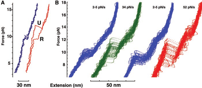
Fig. 11a taken from Ref. (Liphardt et al. 2002) plots an example of the force-extension data which is recorded in unfolding (U) and refolding (R) the RNA hairpin structure. The blue curves represent a slow driving force of 2-5 pN/s while the red curves show a fast driving force of 52 pN/s. Thus we can already see why RNA hairpin structures are ideal candidates for experimental verification of non-equilibrium results; they allow both the quasi-static and non-equilibrium regimes to be accessed. To go from the force-extension data to a value of work simply requires numerically integrating the curves. Fig. 11b shows an ensemble of force-extension curves where the stochastic nature of the fast driving of these small systems is visually apparent.
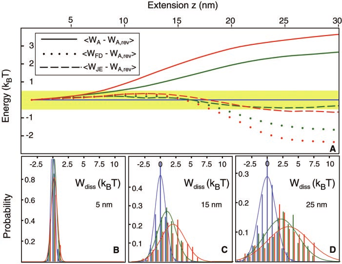
Using the integrated force-extension data, Ref. (Liphardt et al. 2002) then plots the work probability distributions which are shown here in Fig. 12b-d. These plots are analogous to those plotted in Fig. 6 for the toy model where going form sub-figure b-d is analogous to stepping though various \(\lambda\) values in the toy model. Then, similarly to what we have plotted for the toy model in Fig. 12a, they plot the difference between the “actual” free energy difference, which they assume to be the value obtained at the slowest driving rate, and the estimates derived from the JE. They also include an estimate based on a linear fluctuation-dissipation relation (not to be confused with the CFT). Similarly to what we observed in Fig. 7 for the toy model, we see that the JE agrees quite well with the “true” free energy estimate for fast driving rates where the system is driven far from equilibrium.
Experimental verification of the Crooks Fluctuation Theorem

Fig. 13 taken from Ref. (Collin et al. 2005) is analogous to Fig. 8 in The Crooks fluctuation theorem for the toy model where they plot the work distributions for unfolding (forward) and refolding (reverse) the RNA hairpin structure in Fig. 1. Similarly to the work distributions in Fig. 8, we see that as the driving rate is increased, work distributions overlap less, however the point at which the distributions cross remains constant and, according to the CFT, gives the free energy difference between the two configurations.

Remarkably, by applying the CFT the authors of Ref. (Collin et al. 2005) were able to, with statistical significance, distinguish the free energies of the RNA hairpin shown in Fig. 1 and a mutant of the RNA hairpin differing by merely a single swap of one base pair form C-G to G-C. The work distributions of this experiment are shown in Fig. 14a while the log of the ratio between the forward and reverse distributions for the mutant type RNA hairpin are shown in Fig. 14b. Analogously to Fig. 9 for the toy model, we see that the ratio has linear dependence which gives experimental verification of the functional form of the CFT.
Conclusion
We have reviewed two exact results for non-equilibrium thermodynamic systems: the Jarzynski equality and the Crooks fluctuation theorem. We first established the basic thermodynamics background necessary for discussion of these results and introduced the types of non-equilibrium systems for which the JE and CFT apply. We introduced a toy model which captures the relevant features of folding and unfolding and an RNA hairpin. By using MCMC sampling of the toy model, we illustrated the connection between the equilibrium and non-equilibrium regimes and how they manifest in the work probability distributions. We then used this model to explicitly show how each of the JE and CFT are applied to work measurements in order to determine the free energy difference between the two configurations. Finally we discussed the experimental verification of the JE and CFT using optical tweezers. We focused the discussion on the simple toy model so we could concretely illustrate how the relevant non-equilibrium quantities are understood in the context of the JE and CFT in a way that would then match the data from actual experiments.
Now that the JE and CFT are well established tools for understanding non-equilibrium systems, they are routinely used in experiments which probe the free energy landscapes of increasingly more complicated biomolecules such as complex proteins (Shank et al. 2010). Work has continued on generalizing non-equilibrium fluctuation theorems to more settings, unifying the various assumptions, and putting the derivations on more mathematically rigorous ground (Seifert 2012). Furthermore, there is ongoing work to understand the possible computational benefits of extending the results of Jarzynski and Crooks to computational settings where the ability to run multiple fast non-equilibrium molecular simulations in parallel may be more efficient than trying to run fewer simulations which attempt to maintain quasi-static conditions (Dellago and Hummer 2013). Finally, applying the JE and CFT to the non-equilibrium thermodynamics of quantum systems offers the potential for new insights into the behavior of many interesting physical systems where quantum effects cannot be neglected (Ribeiro, Landi, and Semião 2016; Vinjanampathy and Anders 2016).
Appendix: Proof of the Crooks fluctuation theorem
The proof presented here closely follows the one in Crooks’ original paper (Crooks 1999) with exposition that is relevant to the main text of this paper. It’s worth noting that the CFT can be derived in other ways using different formalisms (Seifert 2012). For a good introduction to the notion of non-equilibrium trajectories see Ref. (Zuckerman and Russo 2021).
Before writing down the CFT, we will first require some notation. We denote a path through phase space by \(x(t)\) and, as was used previously, the driving force is parameterized by \(\lambda(t)\). Thus trajectories are unique when we specify both \(x(t)\) and \(\lambda(t)\). The system and bath at a given point in time \(t\) is described by a phase space distribution \(\rho(x_t)\). We then introduce a quantity called the entropy production defined on the level of a single trajectory that takes phase space distributions \(\rho(x_{-\tau})\to\rho(x_{+\tau})\) from \(-\tau\) to \(\tau\) by
\begin{align} \label{eq:ent-prod} \omega_F &= \ln(\rho(x_{-\tau})) - \ln(\rho(x_{+\tau})) - \beta Q\bqty{x(t), \lambda(t)} \end{align}where the notation \(Q\bqty{x(t), \lambda(t)}\) denotes that heat \(Q\) dissipated to the bath is a functional of the path through phase space. We will denote the entropy production in the reverse direction from \(\rho(x_{+\tau})\to\rho(x_{-\tau})\) by \(\omega_R\). Notably \(\omega\) is dependent not only on the initial and final distributions, but the path through phase space due to \(Q\) being a functional. The entropic terms in Eq. \eqref{eq:ent-prod} are of the form \(-\ln(\rho(x))\) since \(\omega\) is defined for a single stochastic trajectory whereas for an ensemble of systems the entropy is given by the usual expression of \(S(x) = -k_B \sum_x \rho(x)\ln\rho(x)\). In other words it is changes in the logarithm of the phase space distribution which cause changes in the entropy of the ensemble since the ensemble itself must always form a complete sample space.
Stochastic dynamics assumes Markovian, or memoryless, behavior which can be summarized, in the discrete case, as
\begin{align} \label{eq:markov} \Pr\bqty{x(t + \Delta t)=b\;|\; x(0)=a_0,\; x(1) = a_1,\;\ldots,\; x(t) = a_t} = \Pr\bqty{x(t + \delta t)\;=b|\; x(t)=a_t}\;. \end{align}Note that when stating Eq. \eqref{eq:markov}, we are implicitly assuming that we condition both sides on the same deterministic path of \(\lambda(t)\). In addition to assuming Markovian dynamics, we will also require microscopic reversibility which can be stated as
\begin{align} \label{eq:micro-rev} \frac{\Pr\bqty{x(+t)|\lambda(+t)}}{\Pr\bqty{\bar{x}(-t)|\bar{\lambda}(-t)}} &= \exp{-\beta Q\bqty{x(+t),\lambda(+t)}} \end{align}where \(\bar{x}(-t) = x(t)\) and \(\lambda(-t) = \lambda(t)\) and thus \(\bar{x}\) and \(\bar{\lambda}\) represent time reversal of each path. This statement of macroscopic reversibility can be thought of as the stochastic trajectory statement of the second law as it relates the probability of trajectories to the change in heat of the bath, which is still assumed to be large and at constant temperature. Thus the change in heat is directly related to entropy dissipated by the bath, even though at this microscopic trajectory level, the system may not remain in thermal equilibrium with the bath.
Finally we require the heat \(Q\) to be odd under time reversal so
\begin{align} Q\bqty{x(+t),\lambda(+t))} &= -Q\bqty{\bar{x}(-t),\bar{\lambda}(-t))} \end{align}along with requiring that the entropy production \(\omega\) also be odd under time reversal \(\omega_F = -\omega_R\). This is equivalent to requiring that
\begin{align} \label{eq:rho-rev} \rho(x_{+\tau}) = \rho(\bar{x}_{+\tau})\quad\text{and}\quad \rho(\bar{x}_{-\tau}) = \rho(x_{-\tau}) \end{align}meaning that the phase space distribution at the end of the forward process is the same as the one at the start of the reverse process. This requirement should sound familiar from The Jarzynski equality, but we note that this is more general, since we’ve not assumed either \(\rho(x_{-\tau})\) or \(\rho(x_{+\tau})\) must be in equilibrium. This generalization of this assumption is how the CFT can also be applied to NESS.
Now we are ready to prove the CFT. We start by substituting Eq. \eqref{eq:ent-prod} into Eq. \eqref{eq:micro-rev} for the forward process then use Eq. \eqref{eq:rho-rev}
\begin{align} \frac{\Pr\bqty{x(+t)|\lambda(+t)}}{\Pr\bqty{\bar{x}(-t)|\bar{\lambda}(-t)}} &= \exp{\omega_F - \ln(\rho(x_{-\tau})) + \ln(\rho(x_{+\tau}))} = e^{\omega_F}\frac{\rho(x_{+\tau})}{\rho(x_{-\tau})} \end{align}which then gives us
\begin{align} \label{eq:crooks-eq7} \frac{\rho(x_{-\tau})\Pr\bqty{x(+t)|\lambda(+t)}} {\rho(\bar{x}_{+\tau})\Pr\bqty{\bar{x}(-t)|\bar{\lambda}(-t)}} = e^{+\omega_F}\; . \end{align}Now we want to write down the probability distribution for entropy production in the forward direction. We can accomplish this by writing it as an average of a delta function \(\delta(\omega - \omega_F)\) where we average over all phase-space paths which start with \(\rho(x_{-\tau})\) and end with \(\rho(x_{+\tau})\). Since we will need to perform functional integration over the path \(x(t)\), we will represent the functional integrand over all paths as \(\mathcal{D}[x(t)]\). Then we write the integral as
\begin{align} \label{eq:crooks-int} P_F(\omega) &= \expval{\delta(\omega - \omega_F)} \nonumber \\&= \int\int\int_{x_{-\tau}}^{x_{+\tau}}\rho(x_{-\tau}) \Pr\bqty{x(+t)|\lambda(+t)} \delta(\omega - \omega_F) \mathcal{D}[x(t)]\dd{x_{-\tau}}\dd{x_{+\tau}} \end{align}We read this integral as first performing functional integration over all paths \(x(t)\) weighted by their probability, given the parameterized drive \(\lambda(t)\). This leads to some final phase space configuration \(\rho(x_{+\tau})\). The delta function constrains the endpoint distributions \(\rho(x_{-\tau})\) and \(\rho(x_{+\tau})\) to be those consistent with the value of \(\omega\) we want the probability of when we perform the final two normal integrations over \(\dd{x_{-\tau}}\) and \(\dd{x_{-\tau}}\) (note that the fact that \(Q\) is a functional in \(\omega_F\) means it was integrated out previously).
To continue with the proof of the CFT, we proceed by substituting Eq. \eqref{eq:crooks-eq7} into Eq. \eqref{eq:crooks-int} which gives us
\begin{align} P_F(\omega) &= \int\int\int_{x_{-\tau}}^{x_{+\tau}}\rho(\bar{x}_{+\tau}) \mathcal{P}\bqty{\bar{x}(-t)|\bar{\lambda}(-t)} \delta(\omega - \omega_F)e^{+\omega_F}\mathcal{D}[x(t)]\dd{x_{-\tau}}\dd{x_{+\tau}} \\&= e^{+\omega_F}\int\int\int_{x_{-\tau}}^{x_{+\tau}}\rho(\bar{x}_{+\tau}) \mathcal{P}\bqty{\bar{x}(-t)|\bar{\lambda}(-t)} \delta(\omega + \omega_R)\mathcal{D}[x(t)]\dd{x_{-\tau}}\dd{x_{+\tau}} \\&= e^{+\omega_F} \expval{\delta(\omega + \omega_R)}_R \\&= e^{+\omega_F} P_R(-\omega) \end{align}and so we have derived the Crook fluctuation theorem
\begin{align} \label{eq:crooks} \frac{P_F(+\omega)}{P_R(-\omega)} &= e^{+\omega_F} \end{align}
We now turn our attention to deriving Eq. \eqref{eq:crooks-under-je} which means understanding what the entropy production quantity Eq. \eqref{eq:ent-prod} represents under the setting for which the JE applies.
Recall that the setting for which the JE applies assumes that the system starts in equilibrium at \(t=-\tau\) and thus the drive must be constant \(\lambda(t) = \lambda_0\) for \(t<-\tau\).
Then the arbitrary drive is applied for \(-\tau
which substituting into Eq. \eqref{eq:crooks}, suppressing the functional argument to \(W\), and reminding ourselves to flip the sign on \(\Delta F\) for the reverse path, we find
\begin{align} \frac{P_F(-\beta\Delta F + \beta W)}{P_R(-\beta\Delta F - \beta W))} &= e^{-\beta(\Delta F + \beta W)} \end{align}However, since \(\beta \Delta F\) is not a functional but rather just a constant offset for the stochastic variable \(W\), we can drop it leaving us with Eq. \eqref{eq:crooks-under-je}.
Appendix: Julia code reproducing Crooks’ original NESS toy model
The following Julia code implements the toy model in Crooks original paper (Crooks 1999).
using Plots, LaTeXStrings
default(fontfamily="Computer Modern", size=(400, 300),
        guidefontsize=10, tickfontsize=8, legendfontsize=8, markersize=3,
        framestyle=:box, tick_direction=:out, label=nothing)

β = 1/5
H = [15:-1:0; 0:1:15]
step(x0, dir) = mod(x0 + dir - 1, 32) + 1
drive_step(i, x0) = (mod(i, 8) == 0) ? step(x0, -1) : x0

function metropolis_step(x0)
    x1 = step(x0, rand((-1,0,1)))
    ΔE = H[x1] - H[x0]
    if ΔE < 0 || rand() < exp(-β*ΔE)
        return x1
    else
        return x0
    end
end

function run_equilibrium(trials)
    xs = zeros(Int64, trials)
    xs[1] = 1
    for i=2:trials
        xs[i] = metropolis_step(xs[i-1])
    end
    return xs
end

function run_ness(trials)
    xs = zeros(Int64, trials)
    xs[1] = 1
    for i=2:trials
        xs[i] = metropolis_step(drive_step(i, xs[i-1]))
    end
    return xs
end

function run_one(init_ensemble, Δt)
    x0 = rand(init_ensemble)
    w, Q = 0, 0
    for i=1:Δt
        x1 = drive_step(i, x0)
        w += H[x1] - H[x0]
        x2 = metropolis_step(x1)
        Q += H[x2] - H[x1]
        x0 = x2
    end
    return w, Q
end

function run(init_ensemble, Δt, N)
    ws, Qs = zeros(Int64, N), zeros(Int64, N)
    for i=1:N
        ws[i], Qs[i] = run_one(init_ensemble, Δt)
    end
    Δt, ws, Qs
end

function plot_it!(Δt, data)
    xs = minimum(data):maximum(data)
    ys = map(n -> count(x -> x==n, data)/length(data), xs)
    #plot!(xs, ys, label="Δt=$(Δt)")
    plot!(β*xs, ys, label="Δt=$(Δt)")
end

plot_work!((Δt, ws, Qs)) = plot_it!(Δt, ws)
plot_heat!((Δt, ws, Qs)) = plot_it!(Δt, -Qs)
This actually does the computationally expensive task of generating all the trajectories.
@time begin
    ensemble = run_equilibrium(2^20)
    equil = [run(ensemble, Δt, 2^20) for Δt in [128, 256, 512, 1024, 2048]]
end;
@time begin
    ensemble = run_ness(2^20)
    ness = [run(ensemble, Δt, 2^20) for Δt in [128, 256, 512, 1024, 2048]]
end;
848.510151 seconds (11.64 G allocations: 173.591 GiB, 1.59% gc time, 0.01% compilation time)
893.518962 seconds (11.61 G allocations: 173.234 GiB, 1.56% gc time, 0.00% compilation time)
The following code recreates Fig. 1 from Ref. (Crooks 1999).
N = 2^20
p1 = plot(xlabel=L"x", ylabel=L"P(x)", legend=:none, ylim=(0,0.101))
p2 = twinx()
plot!(p1, map(n -> count(x -> x==n, run_equilibrium(N))/N, 1:32), markershape=:circle)
plot!(p1, map(n -> count(x -> x==n, run_ness(N))/N, 1:32), markershape=:circle)
scatter!(p2, map(x->H[x], 1:32), ylabel=L"E(x)",
         legend=:none, markershape=:hline, markercolor=:black)

The following code recreates Fig. 2 from Ref. (Crooks 1999).
p = plot(xlabel=L"\beta W", ylabel=L"P(\beta W)", ylims=(0,0.065), xlims=(-8, 28))
foreach(plot_work!, equil); p

The following code recreates Fig. 3 from Ref. (Crooks 1999).
p = plot(xlabel=L"-\beta Q", ylabel=L"P(-\beta Q)", ylims=(0,0.065), xlims=(-8, 28))
foreach(plot_heat!, ness); p

Appendix: Julia code implementing the RNA folding inspired toy model
The following Julia code implements the toy model described in The toy model.
β = 1/2

H = [[(i+7):-1:(i-1); (i-1):1:(13+((i-1)÷2)); (13+(i÷2)):-1:14; 14:1:22]
     for i=1:29]
H = reduce(hcat, H)'
Nλ, Ns = size(H)

Z(λ) = sum(exp(-β*H[λ, i]) for i=1:Ns)
F(λ) = -log(Z(λ))/β

function metropolis_step(λ, x0)
    x1 = x0 + rand((-1,0,1))
    (1 <= x1 <= 32) || return x0

    ΔE = H[λ, x1] - H[λ, x0]
    if ΔE < 0 || rand() < exp(-β*ΔE)
        return x1
    else
        return x0
    end
end

function run_equilibrium(λ, trials)
    xs = zeros(Int64, trials)
    xs[1] = 1
    for i=2:trials
        xs[i] = metropolis_step(λ, xs[i-1])
    end
    return xs
end

function run_one(init_ensemble, Δt, λs)
    x0 = rand(init_ensemble)
    W, Q, X = (zeros(Int64, length(λs)) for _=1:3)
    for j=2:length(λs)
        W[j] = H[λs[j], x0] - H[λs[j-1], x0]
        for i=1:Δt
            x1 = metropolis_step(λs[j], x0)
            Q[j] += H[λs[j], x1] - H[λs[j], x0]
            x0 = x1
        end
        X[j] = x0
    end
    return W, Q, X
end

function run(init_ensemble, Δt, λs, N)
    Ws, Qs, xs = (zeros(Int64, (N, length(λs))) for _=1:3)
    for i=1:N
        Ws[i,:], Qs[i,:], xs[i,:] = run_one(init_ensemble, Δt, λs)
    end
    return Δt, Ws, Qs, xs
end

jarzynski(Ws) = -(1/β)*log(sum(map(W -> exp(-β*W), Ws))/length(Ws))

function hist(data, λ)
    data = sum(data[:,1:λ], dims=2)
    xs = minimum(data):maximum(data)
    ys = map(n -> count(x -> x==n, data)/length(data), xs)
    return β*xs, ys
end
This actually does the computationally expensive task of generating all the trajectories.
ensemble = run_equilibrium(1, 2^18)
fwd = [@time run(ensemble, Δt, 1:Nλ, 2^N) for (Δt, N) in
           [(4, 18), (64, 15), (1024, 12)]];
ensemble = run_equilibrium(Nλ, 2^18)
rev = [@time run(ensemble, Δt, Nλ:-1:1, 2^N) for (Δt, N) in
           [(4, 18), (64, 15), (1024, 12)]];
 5.390360 seconds (93.15 M allocations: 1.757 GiB, 4.46% gc time, 0.03% compilation time)
 9.292353 seconds (187.04 M allocations: 2.833 GiB, 2.48% gc time)
18.598332 seconds (374.85 M allocations: 5.591 GiB, 2.32% gc time)
 5.342675 seconds (93.19 M allocations: 1.758 GiB, 2.52% gc time)
 9.495887 seconds (187.05 M allocations: 2.833 GiB, 3.13% gc time)
18.955520 seconds (374.86 M allocations: 5.592 GiB, 2.07% gc time)
This sets up prettier plotting defaults.
using Plots, LaTeXStrings, Printf
import Statistics: mean

default(fontfamily="Computer Modern", size=(400, 300), markersize=3,
        guidefontsize=10, tickfontsize=8, legendfontsize=8,  annotationfontsize=10,
        framestyle=:box, tick_direction=:out, label=nothing)

Δt_to_i(Δt) = findfirst(isequal(Δt), [4, 64, 1024])
This creates Fig. 4.
plot(xlabel=L"\lambda", ylabel=L"F_\lambda")
println(β*(F(Nλ) - F(1)))
scatter!([F(λ) for λ=1:Nλ])
This creates Fig. 3.
function plot_equilibrium(λ; N=2^20)
    p = plot(ylim=(-0.001, 0.21), dpi=300)
    annotate!(16, 0.18, L"\lambda=%$(λ)")
    pr = [exp(-β*H[λ, x]) for x=1:Ns] ./ Z(λ)
    plot!(pr)
    scatter!(map(n -> count(x -> x==n, run_equilibrium(λ, N))/N, 1:Ns),
           ylabel=L"P(x)", xlabel=L"x", legend=:none, markershape=:circle)
    scatter!(twinx(), map(x -> H[λ, x], 1:Ns), ylim=(-0.5,36.5),
             ylabel=L"E(x)", legend=:none, mc=:black, shape=:hline, markersize=6)
    plot!(framestyle=:box, xlims=(-0.5, 32.5), xticks=0:2:32,)
    p
end

p1 = plot_equilibrium(1)
p2 = plot_equilibrium(15)
p3 = plot_equilibrium(Nλ)
foreach(p -> plot!(p, xformatter=:none, xlabel=""), [p1, p2])
plot(p1, p2, p3, size=(500, 600), layout=(3,1))
This creates Fig. 5.
function plot_noneq_all(λ)
    plot_noneq!((Δt, Ws, Qs, xs)) =
        plot!(map(n -> count(x -> x==n, xs[:,λ])/length(xs[:,λ]), 1:Ns),
              label="Δt=$(Δt)", color=Δt_to_i(Δt), marker=:circle, legend=:none)

    p = plot(xlable=L"x", ylabel=L"P(x)", ylim=(-0.01,0.21), dpi=300)
    annotate!(16, 0.16, L"\lambda=%$(λ)")
    plot!([exp(-β*H[1, x]) for x=1:Ns] ./ Z(1), ls=:dash, label=L"\lambda=1")
    plot!([exp(-β*H[λ, x]) for x=1:Ns] ./ Z(λ), ls=:dash, label="equilibrium", color=3)
    foreach(plot_noneq!, fwd)
    scatter!(twinx(), map(x -> H[λ, x], 1:Ns), ylim=(-0.5,36.5),
             ylabel=L"E(x)", legend=:none, mc=:black, shape=:hline, markersize=6)
    plot!(framestyle=:box, xlims=(-0.5, 32.5), xticks=0:2:32,)
    p
end

p1 = plot_noneq_all(15)
p2 = plot_noneq_all(22)
p3 = plot_noneq_all(Nλ)
foreach(p -> plot!(p, xformatter=:none, xlabel=""), [p1, p2])
p4 = plot(legend=:top, framestyle=:none, legend_columns=-1, margin=(0,:px))
foreach(i -> plot!(p4, [1], label=p1[1][i][:label], ls=p1[1][i][:linestyle],
                   c=p1[1][i][:seriescolor],
                   marker=p1[1][i][:markershape]), 1:5)
l = @layout [a{0.01h}; grid(3,1)]
plot(p4, p1, p2, p3, size=(500, 650), layout=l,  right_margin=(30, :px))
This creates Fig. 6.
function subplot_work(λ, ylim)
    plot_work_!((Δt, Ws, Qs, xs)) = plot!(hist(Ws, λ)...; color=Δt_to_i(Δt), label="Δt=$(Δt)")
    p = plot(xlabel=L"\beta W", ylabel=L"P(\beta W)", dpi=300,
             xlims=(1.5,14.5), xticks=1:15, ylims=(-0.01,ylim), legend=:none)
    annotate!(3.4, ylim - 0.2*ylim, L"\lambda=%$(λ)")
    foreach(plot_work_!, fwd)
    p
end

p1 = subplot_work(15, 1.0)
p2 = subplot_work(22, 1.0)
p3 = subplot_work(Nλ, 0.35)
foreach(p -> plot!(p, xformatter=:none, xlabel="", bottom_margin=(-20, :px)), [p1, p2])
p4 = plot(legend=:top, framestyle=:none, legend_columns=-1,
          margin=(0,:px), bottom_margin=(-15, :px))
foreach(i -> plot!(p4, [1], label=p1[1][i][:label]), 1:3)
plot(p4, p1, p2, p3, size=(500, 650), layout=@layout [a{0.01h}; grid(3,1)])
This creates Fig. 7.
function plot_work_diff((Δt, Ws, Qs, xs), ΔF)
    works = [sum(Ws[:,1:λ], dims=2) for λ=1:Nλ]
    p = plot!(map(jarzynski, works) - ΔF, color=Δt_to_i(Δt),
              label=L"\Delta t=" * (@sprintf "%4d" Δt) *
                  L" , \Delta \tilde{F}_{\lambda=15} =" *
                  (@sprintf "%.3f" β*jarzynski(works[end])))
    plot!(map(mean, works) - ΔF, ls=:dash, c=p[1][end][:seriescolor])
end
plot_work_diff_fwd(d) = plot_work_diff(d, map(λ -> F(λ) - F(1), 1:Nλ))
plot_work_diff_rev(d) = plot_work_diff(d, map(λ -> F(λ) - F(Nλ), Nλ:-1:1))

p = plot(xlabel=L"\lambda", ylabel=L"\Delta\tilde{F}_\lambda - \Delta F_\lambda",
         legend=:topleft, ylim=(-0.2, 5))
foreach(plot_work_diff_fwd, fwd); p
#foreach(plot_work_diff_rev, rev); p
This creates Fig. 8.
function plot_work_both!((Δt_f, Ws_f, Qs_f), (Δt_r, Ws_r, Qs_r))
    p = plot!(hist(Ws_f, Nλ)...; label="Δt=$(Δt_f)", color=Δt_to_i(Δt_f))
    plot!(hist(-Ws_r, Nλ)...; ls=:dash, c=p[1][end][:seriescolor])
end
p = plot(xlabel=L"\beta W", ylabel=L"P_F(\beta W), P_R(-\beta W)",
         ylim=(-0.01, 0.34), legend=:top)
foreach(plot_work_both!, fwd, rev); p
This creates Fig. 9.
function plot_crooks!((Δt_f, Ws_f, Qs_f), (Δt_r, Ws_r, Qs_r))
    function hist_(xs, data)
        data = sum(data[:,1:Nλ], dims=2)
        ys = map(n -> count(x -> x==n, data)/length(data), xs)
        return ys
    end
    xs = -100:100
    #xs = -10:60

    ys_f = hist_(xs, Ws_f)
    ys_r = hist_(xs, -Ws_r)

    ys = log.(ys_f ./ ys_r)
    xs = xs[isfinite.(ys)]
    ys = ys[isfinite.(ys)]
    xs = β*xs

    M = [ones(length(xs)) xs]
    a, b = M \ ys

    #p = scatter!(β*xs, ys, label=L"\Delta t=" * (@sprintf "%4d" Δt_f) *", a=" *
    #             (@sprintf "%.3f" b/β) * ", b=" * (@sprintf "%.3f" -β*a/b))
    p = scatter!(xs, ys, color=Δt_to_i(Δt_f),
                 label=L"\Delta t=" * (@sprintf "%4d" Δt_f) * ", a=" *
                 (@sprintf "%.2f" b) * ", b=" * (@sprintf "%.2f" -a) * L", \Delta\tilde{F}=" *
                 (@sprintf "%.2f" -mean(ys - xs)))
    plot!(xs, a .+ b .* xs, ls=:dash, c=p[1][end][:seriescolor])
end

p = plot(xlabel=L"\beta W", ylabel=L"\log[P_F(\beta W)/P_R(\beta W)]")
foreach(plot_crooks!, fwd, rev); p
Appendix: Potential plotting code
using Plots, LaTeXStrings
default(fontfamily="Computer Modern", plot_titlefontsize=10, titlefontsize=10,
        guidefontsize=10, tickfontsize=8, legendfontsize=8, annotationfontsize=12,
        markersize=3, framestyle=:box, tick_direction=:out, label=nothing)

plot(size=(400,300) , grid=:false, framestyle=:origin, ticks=:none,
     right_margin=(20, :px), top_margin=(20, :px))
x = collect(0:0.01:4)
y(a; x0=2) = @. a*x^2 - 3*(x-x0)^2 + (x-x0)^4 + 2.3
plot!(x, [y(.2), y(0), y(-.2)])
annotate!(0.8, 2.2, "folded")
annotate!(3, 3.8, "unfolded")
annotate!(3.7, 10.5, "external force")
plot!([4.2,4.2], [10,3], arrow = :arrow, lw=2, lc=:black)
annotate!(4.5, 0, L"x")
annotate!(0, 11.0, L"E(x)")